Analytical Chemistry
May 1, 1996

Analytical Chemistry 1996, (68) 305A-309A

Copyright © 1996 by the American Chemical Society.

A Practical Guide to Analytical Method Validation

Doing a thorough method validation can be tedious, but the consequences of not doing it right are wasted time, money, and resources

The ability to provide timely, accurate, and reliable data is central to the role of analytical chemists and is especially true in the discovery, development, and manufacture of pharmaceuticals. Analytical data are used to screen potential drug candidates, aid in the development of drug syntheses, support formulation studies, monitor the stability of bulk pharmaceuticals and formulated products, and test final products for release. The quality of analytical data is a key factor in the success of a drug development program. The process of method development and validation has a direct impact on the quality of these data.

Although a thorough validation cannot rule out all potential problems, the process of method development and validation should address the most common ones. Examples of typical problems that can be minimized or avoided are synthesis impurities that coelute with the analyte peak in an HPLC assay; a particular type of column that no longer produces the separation needed because the supplier of the column has changed the manufacturing process; an assay method that is transferred to a second laboratory where they are unable to achieve the same detection limit; and a quality assurance audit of a validation report that finds no documentation on how the method was performed during the validation.

Problems increase as additional people, laboratories, and equipment are used to perform the method. When the method is used in the developer's laboratory, a small adjustment can usually be made to make the method work, but the flexibility to change it is lost once the method is transferred to other laboratories or used for official product testing. This is especially true in the pharmaceutical industry, where methods are submitted to regulatory agencies and changes may require formal approval before they can be implemented for official testing. The best way to minimize method problems is to perform adequate validation experiments during development.

What is method validation?
Method validation is the process of proving that an analytical method is acceptable for its intended purpose. For pharmaceutical methods, guidelines from the United States Pharmacopeia (USP) (1), International Conference on Harmonisation (ICH) (2), and the Food and Drug Administration (FDA) (3, 4) provide a framework for performing such validations. In general, methods for regulatory submission must include studies on specificity, linearity, accuracy, precision, range, detection limit, quantitation limit, and robustness.

Although there is general agreement about what type of studies should be done, there is great diversity in how they are performed (5). The literature contains diverse approaches to performing validations (as in References 6--10). This Report presents an approach to performing validation studies that encompasses much of the current literature and provides practical guidance. This approach should be viewed with the understanding that validation requirements are continually changing and vary widely, depending on the type of drug being tested, the stage of drug development, and the regulatory group that will review the drug application. For our purposes, we will discuss validation studies as they apply to chromatographic methods, although the same principles apply to other analytical techniques.

In the early stages of drug development, it is usually not necessary to perform all of the various validation studies. Many researchers focus on specificity, linearity, accuracy, and precision studies for drugs in the preclinical through Phase II (preliminary efficacy) stages. The remaining studies are performed when the drug reaches the Phase III (efficacy) stage of development and has a higher probability of becoming a marketed product.

The process of validating a method cannot be separated from the actual development of the method conditions, because the developer will not know whether the method conditions are acceptable until validation studies are performed. The development and validation of a new analytical method may therefore be an iterative process. Results of validation studies may indicate that a change in the procedure is necessary, which may then require revalidation. During each validation study, key method parameters are determined and then used for all subsequent validation steps. To minimize repetitious studies and ensure that the validation data are generated under conditions equivalent to the final procedure, we recommend the following sequence of studies.

Establish minimum criteria
The first step in the method development and validation cycle should be to set minimum requirements, which are essentially acceptance specifications for the method. A complete list of criteria should be agreed on by the developer and the end users before the method is developed so that expectations are clear.

For example, is it critical that method precision (RSD) be „ 2%? Does the method need to be accurate to within 2% of the target concentration? Is it acceptable to have only one supplier of the HPLC column used in the analysis? During the actual studies and in the final validation report, these criteria will allow clear judgment about the acceptability of the analytical method.

Examples of minimum criteria are provided throughout this article that indicate practical ways to evaluate the acceptability of data from each validation study. The statistics generated for making comparisons are similar to what analysts will generate later in the routine use of the method and therefore can serve as a tool for evaluating later questionable data. More rigorous statistical evaluation techniques are available and should be used in some instances, but these may not allow as direct a comparison for method troubleshooting during routine use.

Demonstrate specificity
For chromatographic methods, developing a separation involves demonstrating specificity, which is the ability of the method to accurately measure the analyte response in the presence of all potential sample components. The response of the analyte in test mixtures containing the analyte and all potential sample components (placebo formulation, synthesis intermediates, excipients, degradation products, process impurities, etc.) is compared with the response of a solution containing only the analyte. Other potential sample components are generated by exposing the analyte to stress conditions sufficient to degrade it to 80-90% purity. For bulk pharmaceuticals, stress conditions such as heat (50 |AoC), light (600 FC), acid (0.1 N HCl), base (0.1 N NaOH), and oxidant (3% H2O2) are typical. For formulated products, heat, light, and humidity (85%) are often used.

The resulting mixtures are then analyzed, and the analyte peak is evaluated for peak purity and resolution from the nearest eluting peak. If an alternate chromatographic column is to be allowed in the final method procedure, it should be identified during these studies. Once acceptable resolution is obtained for the analyte and potential sample components, the chromatographic parameters, such as column type, mobile-phase composition, flow rate, and detection mode, are considered set.

An example of specificity criteria for an assay method is that the analyte peak will have baseline chromatographic resolution of at least 1.5 from all other sample components. If this cannot be achieved, the unresolved components at their maximum expected levels will not affect the final assay result by more than 0.5%. An example of specificity criteria for an impurity method is that all impurity peaks that are „ 0.1% by area will have baseline chromatographic resolution from the main component peak(s) and, where practical, will have resolution from all other impurities.

Demonstrate linearity
A linearity study verifies that the sample solutions are in a concentration range where analyte response is linearly proportional to concentration. For assay methods, this study is generally performed by preparing standard solutions at five concentration levels, from 50 to 150% of the target analyte concentration. Five levels are required to allow detection of curvature in the plotted data. The standards are evaluated using the chromatographic conditions determined during the specificity studies.

Standards should be prepared and analyzed a minimum of three times. The 50 to 150% range for this study is wider than what is required by the FDA guidelines. In the final method procedure, a tighter range of three standards is generally used, such as 80, 100, and 120% of target; and in some instances, a single standard concentration is used.

Validating over a wider range provides confidence that the routine standard levels are well removed from nonlinear response concentrations, that the method covers a wide enough range to incorporate the limits of content uniformity testing, and that it allows quantitation of crude samples in support of process development. For impurity methods, linearity is determined by preparing standard solutions at five concentration levels over a range such as 0.05-2.5 wt%.

Acceptability of linearity data is often judged by examining the correlation coefficient and y-intercept of the linear regression line for the response versus concentration plot. A correlation coefficient of > 0.999 is generally considered as evidence of acceptable fit of the data to the regression line. The y-intercept should be less than a few percent of the response obtained for the analyte at the target level.

Although these are very practical ways of evaluating linearity data, they are not true measures of linearity (11, 12). These parameters, by themselves, can be misleading and should not be used without a visual examination of the response versus concentration plot. An example of how the use of correlation coefficients can be misleading can be seen in data from an HPLC method for quantitation of mannitol. This method uses an internal standard, so the data are recorded as peak area ratios (mannitol area/internal standard area). Figure 1 is a plot of mannitol peak area ratio versus mannitol concentration for standards analyzed by the method. Although the correlation coefficient of the linear regression is > 0.999 (top), the plot indicates small deviations from linearity at low and high concentrations. An alternate way of evaluating the data is to plot response factor [(peak area ratio \N y intercept)/concentration)] versus concentration (also shown in Figure 1).

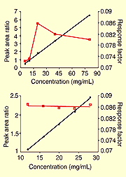
Figure 1. Peak area ratio (circles) and response factor (squares) versus concentration for mannitol.

(Top) Concentration range is 5-80 mg/mL. For peak area ration line, y=0.09775 + 0.080569x and correlatin coefficiant = 0.99952. (Bottom) Concentration range is 12-28 mg/mL. For peak area ratio line, y-0.027 + 0.08625x and correlation coefficiant = 0.99965.

If an equivalent response was obtained at each concentration, the data points would form a straight line with a zero slope. The response factors plotted in Figure 1(top) vary greatly over the range and fall only within 15% of the target concentration. A second set of mannitol data, over a narrower range of concentrations, is shown in Figure 1(bottom). The response factors for all concentrations in this range are within 1.5% of the target concentration response. The near-zero slope of the response factor plot indicates that a linear response is obtained over this concentration range.

At the completion of linearity studies, the appropriate concentration range for the standards and the injection volume should be set for all subsequent studies.

An example of a linearity criteria for an assay method is that the correlation coefficient for each of three curves (five concentration levels each) will be „ 0.99 for the range 80\N120\% of the target concentration. The y-intercept will be „ 2% of the target concentration response. An alternate criteria is that a plot of response factor versus concentration will show all values within 2.5% of the target-level response factor for concentrations between 80 and 120% of the target concentration. For an impurity method, the correlation coefficient for each of three curves (five concentration levels each) will be „ 0.98 for the range 0.--1 2.5% of the main component concentration. The y-intercept will be „ 10% of the response produced for a 2.5 wt% impurity. An alternate criteria is that a plot of response factor versus concentration will show all values within 5% of the mean response factor for concentrations „ 0.5 wt% and within 10% of the mean response factor for concentrations „ 0.5 wt%.

Demonstrate accuracy
The accuracy of a method is the closeness of the measured value to the true value for the sample. Accuracy is usually determined in one of four ways. First, accuracy can be assessed by analyzing a sample of known concentration and comparing the measured value to the true value. National Institute of Standards and Technology (NIST) reference standards are often used; however, such a well-characterized sample is usually not available for new drug-related analytes. The second approach is to compare test results from the new method with results from an existing alternate method that is known to be accurate. Again, for pharmaceutical studies, such an alternate method is usually not available.K/p %The third and fourth approaches are based on the recovery of known amounts of analyte spiked into sample matrix. The third approach, which is the most widely used recovery study, is performed by spiking analyte in blank matrices. For assay methods, spiked samples are prepared in triplicate at three levels over a range of 50--150% of the target concentration. If potential impurities have been isolated, they should be added to the matrix to mimic impure samples. For impurity methods, spiked samples are prepared in triplicate at three levels over a range that covers the expected impurity content of the sample, such as 0.1--2.5 wt%. The analyte levels in the spiked samples should be determined using the same quantitation procedure as will be used in the final method procedure (i.e., same number and levels of standards, same number of sample and standard injections, etc.). The percent recovery should then be calculated.

The fourth approach is the technique of standard additions, which can also be used to determine recovery of spiked analyte. This approach is used if it is not possible to prepare a blank sample matrix without the presence of the analyte. This can occur, for example, with lyophilized material, in which the speciation in the lyophilized material is significantly different when the analyte is absent.

An example of an accuracy criteria for an assay method is that the mean recovery will be 100 + 2% at each concentration over the range of 80--120% of the target concentration. For an impurity method, the mean recovery will be within 0.1% absolute of the theoretical concentration or 10% relative, whichever is greater, for impurities in the range of 0.1--2.5 wt%.

Determine the range
The range of an analytical method is the concentration interval over which acceptable accuracy, linearity, and precision are obtained. In practice, the range is determined using data from the linearity and accuracy studies. Assuming that acceptable linearity and accuracy (recovery) results were obtained as described earlier, the only remaining factor to be evaluated is precision. This precision data should be available from the triplicate analyses of spiked samples in the accuracy study.

Figure 2 illustrates how precision may change as a function of analyte level. The %RSD values for ethanol quantitation by GC increased significantly as the concentration decreased from 1000 ppm to 10 ppm. Higher variability is expected as the analyte levels approach the detection limit for the method. The developer must judge at what concentration the imprecision becomes too great for the intended use of the method.

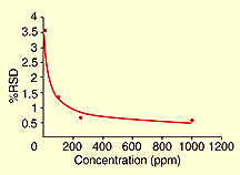
Figure 2. %RSD versus concentration for a GC headspace analysis of ethanol.

An example of range criteria for an assay method is that the acceptable range will be defined as the concentration interval over which linearity and accuracy are obtained per previously discussed criteria and that yields a precision of „ 3% RSD. For an impurity method, the acceptable range will be defined as the concentration interval over which linearity and accuracy are obtained per the above criteria, and that, in addition, yields a precision of „ 10% RSD.

Determine precision, Round 1
The precision of an analytical method is the amount of scatter in the results obtained from multiple analyses of a homogeneous sample. To be meaningful, the precision study must be performed using the exact sample and standard preparation procedures that will be used in the final method.

The first type of precision study is instrument precision or injection repeatability (3). A minimum of 10 injections of one sample solution is made to test the performance of the chromatographic instrument. The second type is repeatability or intra-assay precision (2). Intra-assay precision data are obtained by repeatedly analyzing, in one laboratory on one day, aliquots of a homogeneous sample, each of which has been independently prepared according to the method procedure. From these precision studies, the sample preparation procedure, the number of replicate samples to be prepared, and the number of injections required for each sample in the final method procedure will be set. Two additional types of precision studies are described later in Round 2.

An example of precision criteria for an assay method is that the instrument precision (RSD) will be „ 1% and the intra-assay precision will be „ 2%. For an impurity method, at the limit of quantitation, the instrument precision will be „ 5% and the intra-assay precision will be „ 10%.

Widen the scope
Once these validation studies are complete, the method developers should be confident in the ability of the method to provide good quantitation in their own laboratories. This result may be sufficient for many methods, especially in the early phases of drug development. The remaining studies should provide greater assurance that the method will work well in other laboratories, where different operators, instruments, and reagents are involved and where it will be used over much longer periods of time.

This is a good time to begin accumulating data for two or more system suitability criteria, which are required prior to routine use of the method to ensure that it is performing appropriately. Typically, the process involves making five injections of a standard solution and evaluating several chromatographic parameters (1) such as resolution, area % reproducibility, number of theoretical plates, and tailing factor.

Establish the detection limit
The detection limit of a method is the lowest analyte concentration that produces a response detectable above the noise level of the system, typically, three times the noise level. The detection limit needs to be determined only for impurity methods in which chromatographic peaks near the detection limit will be observed. The detection limit should be estimated early in the method development-validation process and should be repeated using the specific wording of the final procedure if any changes have been made. It is important to test the method detection limit on different instruments, such as those used in the different laboratories to which the method will be transferred. An example of a detection limit criteria is that, at the 0.05% level, an impurity will have S/N G 3.

Establish the quantitation limit
The quantitation limit is the lowest level of analyte that can be accurately and precisely measured. This limit is required only for impurity methods and is determined by reducing the analyte concentration until a level is reached where the precision of the method is unacceptable. If not determined experimentally, the quantitation limit is often calculated as the analyte concentration that gives S/N = 10. An example of quantitation limit criteria is that the limit will be defined as the lowest concentration level for which an RSD „ 20% is obtained when an intra-assay precision study is performed.

Establish stability
During the earlier validation studies, the method developer gained some information on the stability of reagents, mobile phases, standards, and sample solutions. For routine testing in which many samples are prepared and analyzed each day, it is often essential that solutions be stable enough to allow for delays such as instrument breakdowns or overnight analyses using autosamplers. At this point, the limits of stability should be tested. Samples and standards should be tested over at least a 48-h period, and quantitation of components should be determined by comparison to freshly prepared standards. If the solutions are not stable over 48 h, storage conditions or additives should be identified that can improve stability.

An example of stability criteria for assay methods is that sample and standard solutions and the mobile phase will be stable for 48 h under defined storage conditions. Acceptable stability is „ 2% change in standard or sample response, relative to freshly prepared standards. The mobile phase is considered to have acceptable stability if aged mobile phase produces equivalent chromatography (capacity factors, resolution, or tailing factor) and assay results are within 2% of the value obtained with fresh mobile phase.

For impurity methods, the sample and standard solutions and mobile phase will be stable for 48 h under defined storage conditions. Acceptable stability is „ 20% change in standard or sample response at the limit of quantitation, relative to freshly prepared standards. The mobile phase is considered to have acceptable stability if aged mobile phase produces equivalent chromatography and if impurity results at the limit of quantitation are within 20% of the values obtained with fresh mobile phase.

Establish precision, Round 2
The remaining precision studies comprise much of what historically has been called ruggedness. Intermediate precision (2) is the precision obtained when the assay is performed by multiple analysts, using multiple instruments, on multiple days, in one laboratory. Different sources of reagents and multiple lots of columns should also be included in this study. Intermediate precision results are used to identify which of the above factors contribute significant variability to the final result.

The last type of precision study is reproducibility (2), which is determined by testing homogeneous samples in multiple laboratories, often as part of interlaboratory crossover studies. The evaluation of reproducibility results often focuses more on measuring bias in results than on determining differences in precision alone. Statistical equivalence is often used as a measure of acceptable interlaboratory results. An alternative, more practical approach is the use of "analytical equivalence" in which a range of acceptable results is chosen prior to the study and used to judge the acceptability of the results obtained from the different laboratories.

An example of reproducibility criteria for an assay method could be that the assay results obtained in multiple laboratories will be statistically equivalent or the mean results will be within 2% of the value obtained by the primary testing lab. For an impurity method, results obtained in multiple laboratories will be statistically equivalent or the mean results will be within 10% (relative) of the value obtained by the primary testing lab for impurities „ 1wt%, within 25% for impurities from 0.1-1.0 wt%, and within 50% for impurities \h0.1wt%.

Is it robust?
The robustness of a method is its ability to remain unaffected by small changes in parameters such as percent organic content and pH of the mobile phase, buffer concentration, temperature, and injection volume. These method parameters may be evaluated one factor at a time or simultaneously as part of a factorial experiment (13). Obtaining data on the effects of these parameters may allow a range of acceptable values to be included in the final method procedure. For example, if column performance changes over time, adjusting the mobile-phase strength to compensate for changes in the column may be allowed if such data are included in the validation.

An example of robustness criteria is that the effects of the following changes in chromatographic conditions will be determined: methanol content in mobile phase adjusted by + 2%, mobile-phase pH adjusted by + 0.1 pH units, and column temperature adjusted by + 5 |AoC. If these changes are within the limits that produce acceptable chromatography, they will be incorporated in the method procedure.

Doing it right the first time
Performing a thorough method validation can be a tedious process, but the quality of data generated with the method is directly linked to the quality of this process. Time constraints often do not allow for sufficient method validations. Many researchers have experienced the consequences of invalid methods and realized that the amount of time and resources required to solve problems discovered later exceeds what would have been expended initially if the validation studies had been performed properly. We hope that we have provided a guide to help you wend your way efficiently through the method validation maze and eliminate many of the problems common to inadequately validated analytical methods.